View the equipment

Following Becquerel's discovery of X-rays in 1895, other types of radiation were discovered to result from the nuclear decay of certain elements. Much effort went into the study of these radioactive elements, such as Madame Curie's work to isolate the element radium, as well as study of the radioactive emissions themselves. It was soon determined that there were three types of radiation that resulted from the decay of these radioactive elements: alpha particles, which are identical with the nuclei of helium; beta particles, which are identical with electrons; and gamma rays, which are highly energetic photons.

With the advent of nuclear war and the expanded use of nuclear materials in other, more useful ways, there was a great effort in the decades following World War II to determine the effects of radiation on living things, including humans. When it was determined that these radiations were a serious health threat, steps were taken to both shield people from unnecessary radiation and to reduce the dosage of diagnostic radiation. These simple experiments will allow you to explore some of the differences of beta particles and gamma rays, and to determine the kind and thickness of shielding necessary to prevent excessive exposure to radiation of various types.

When you have completed this experimental activity you should be able to: define the terms half-life, activity, corrected activity, standard deviation, sample standard deviation, and half-value layer; measure background radiation; correct activity for background; understand the statistical nature of radiation counting; determine the half-value layer for both beta and gamma radiation; and plot data on a semi-log graph.

During the 1920s it was shown that the alpha, beta and gamma radiation came from the nuclei of certain unstable atoms. Many of the very largest nuclei, those with atomic numbers greater than 82, were always unstable. Other, lighter atoms, had both stable and unstable isotopes. Much effort went into the study of which isotopes were unstable, and what kinds of radiation would be emitted by the nuclei in its attempt to find stability.

There is no way in which we can influence the decay of radioactive atoms. We can neither retard their rate of decay by refrigeration or any other means nor accelerate their rate of decay by the use of heat, pressure, etc. Thus, the amount of radioactivity or the number of radioactive atoms which we have on hand at any time is undergoing a consistent, continuous change.

Fortunately, this change in the number of radioactive atoms follows a very orderly process. If we know the number of atoms on hand and their decay constant, we can calculate how many atoms will remain at any future time. If the number of radioactive atoms remaining at any given instant is plotted against time, curves similar to those on page three will be obtained. The decay constant (k) may be obtained from the slope of the curve. The number of nuclei which decay from a sample of N atoms in time t is given by:

Another more common method of expressing the decay of radioactive atoms is the half-life. The half-life of a radioactive isotope is the time required for the disintegration of one-half of the atoms in the original sample. In the graphs shown below, 1000 atoms were present in this sample at zero elapsed time. At the end of one day, 500 atoms were present. The half-life of this particular nuclide is one day. Therefore, after a time interval equal to two half-lives, only one-quarter of the atoms remain, and so on. The half-life t_½ is related to the decay constant k by the simple relation:

The activity of a particular sample is also often expressed in terms of the number of disintegrations per second that occur. However, since the number of atoms in even a very small sample is quite large, the standard unit of activity is the Curie, which is 10¹⁰ disintegrations per second. Many smaller samples will have activities measured as millicuries (mC) or microcuries (µC). Samples used in this laboratory exercise will be on the order of a microcurie or less in activity.

The ability of radiation to penetrate matter depends on the mass of the particle and whether it is charged or neutral. The larger the mass, the shorter the penetration distance of the radiation will be. For example, an alpha particle, with a mass of 4 amu and charge of +2e, is typically stopped by a sheet of paper or a thin sheet of plastic. Beta particles, being lighter but also carrying charge, will penetrate paper and thin plastic, but be stopped by thicker plastic or thin lead shielding. Gamma rays, which are massless and electrically neutral, have a much greater penetrating ability, and require thicker lead shielding to stop them.

If a beam of beta particles or gamma rays impinge upon a sheet of absorbing material, some of the radiation will pass on through while some will be absorbed or scattered. As the thickness of the absorber is increased, the fraction of the radiation passing through will decrease. The thickness of absorbers is given in the unit mg/cm². The absorptive power of a material is dependent upon its density and thickness, so the product of these two quantities is given as the total absorber thickness. Thus,

Absorber thickness = (density) * (thickness)

mg/cm² = mg/cm³ * cm

When exactly half the radiation incident upon an absorber is passed through it, the thickness of the absorber is called by the special name of Half-value layer, HVL, or half-thickness, X_½. Since the intensity of radiation is reduced by 50% by passing through one HVL, it will be reduced by another 50%, to only 25% of the original intensity, in passing through a second HVL of absorber. The figure shows this progression as a decreasing exponential curve. However, if the data is plotted as a semilog plot, a linear relationship is found, as in the second figure. By using this relationship, the HVL may be easily extrapolated from the activity vs. absorber thickness data.

Using the Beta source (green disk), place the source on one of the middle shelf locations in the counting chamber under the geiger tube. Changing the location upward will increase the counting rate; moving it downward will decrease the rate. Test it for yourself if you wish, but once you begin recording data for this portion, you need to keep it in the same location.

Make 20 (twenty) one-minute counts of the activity of the beta source. The counter has a built-in timer that stops the counter after a one-minute run. Push the right-hand switch to "Stop," push the middle switch to "Reset," be sure the counter reads all zeros, then push the right-hand switch all the way up to "1-minute count." The counter will automatically begin counting, and stop after one minute. Simply record the count, push the right switch to "Stop," reset and start over. These counts may be recorded on the left half of the attached data sheet, under "Sample # 1." You will observe that the counts are seldom identical, but should be reasonably consistent.

After making 20 counts of the beta source, remove it from the counting chamber and make twenty (20) counts of the background level. Background radiation comes from many sources, from the air we breathe to the concrete blocks we build with to the dirt we walk on. Typically background counts are very low, and you may want to keep an eye on the clock to see when the minute has passed. These counts may be recorded on the right half of the attached data sheet, under "Sample # 2." Once again there will likely be some randomness in the measured counts.

Enter the first set of counts in a spreadsheet. Add the column to find the total counts, and divide that value by 20 to find the mean (average). The second column should be the first column minus the mean. The third column is the square of the second column. Show no more than 2 decimal places in the second and third columns. Find the sums of the second and third columns. Are you surprised by the value of either sum?

Now calculate the standard deviation, which is the square root of the average of the third column. If your data are perfectly random, 68% of the observed values of n (i.e., about 13 out of the 20 observations) should lie within a range of one standard deviation of the mean.  Mathematically, the standard deviation formula reads:

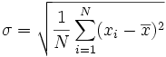
Finally, calculate the sample standard deviation, which is the sum of the third column divided by 19 (one less than the number of observations). The sample standard deviation is calculated in such a way that 68% of the data will fall within the range of one sample standard deviation of the mean, even if the data are not perfectly random. If the data are sufficiently random, the value of the sample standard deviation will equal the standard deviation as the number of observations becomes very large.

Place the Beta source (green disk) in the sample holder, in one of the middle shelves of the counting chamber. Place above it the plastic shelf with the large opening, on which various absorber disks can be placed. Make three one minute counts of the beta source with no absorber in the chamber. Record each count.

Place the thinnest polyethylene absorber, with thickness of 10 mg/cm², on the absorber shelf and take three counts of the beta source, recording the absorber thickness along with each count. Replace the absorber with the next thicker one, and repeat. Use each of the seven polyethylene absorbers, recording absorber thickness and each of the three separate counts with each absorber.

Enter the data in a spreadsheet. Find the average of the three counts for each absorber thickness. Correct the average for background by subtracting the average background count found in part A. Make a logarithmic plot of corrected activity vs. absorber thickness (go to custom types, and choose logarithmic). Include the zero absorber as one of your points. Plot this as data points with no line. Then, fit a linear trendline through the points. What does a linear trendline look like on this graph?  Would you say your data is linear?  Estimate the Half-value Layer (HVL) using this plot. 

Make another column on the spreadsheet that is the common (base 10) log of the corrected activity. Use the function LOG(number,[base]). Make a scatter plot of the data, using absorber thickness as the independent variable and the log(activity) as the dependent variable. 

Then compute the HVL from the slope of the trendline as HVL = -0.3010/slope. Compare the two values of HVL for beta emission, using percent difference. Were you able to make a good estimate from the logarithmic graph?

Use the gamma source (orange disk) in place of the beta source, and make a similar set of counts, using first no absorber, then using the thickest polyethylene absorber (610 mg/cm²), and the four lead absorbers (thickness up to 7200 mg/cm²). Do not use the thinner polyethylene absorbers, as that would be merely a waste of time. You should have three counts for each absorber thickness, just as before.

Analyze this data in the same way you analyzed the absorption data for the beta source. Make the same plot and do the same type of trendline. Find the HVL for the gamma radiation.

Write your conclusions and attach the graphs and data tables to your report. You should comment on whether your data in part A seems to be random (based on a comparison of the standard deviation with the sample standard deviation), and draw conclusions about the relative penetrating ability of beta and gamma radiation based on your HVL values for each. You may wish to comment on the significance of the background radiation in your experimental work.

 Close Window